ArXiv
Preprint
Source Code
Github

Dataset
Hugging Face
How Do AI Models Fold Proteins?
Ever since AlphaFold showed that AI could predict protein structures with atomic accuracy, scientists have asked: how does it actually work? We study this question by opening up ESMFold, a state-of-the-art protein folding model. Our work is the first mechanistic analysis of the folding trunk, the core engine that turns amino acid sequences into 3D structures. We find that the trunk operates in two distinct phases: first assembling a chemical picture of residue interactions, then building the geometric blueprint that determines the final fold. These internal representations are not just interpretable: they can be steered to change the predicted structure.
What is a Protein Structure?
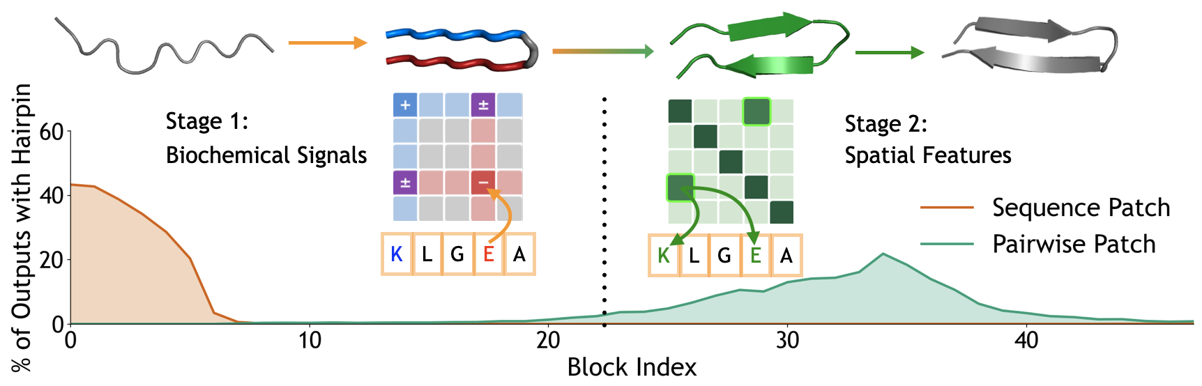
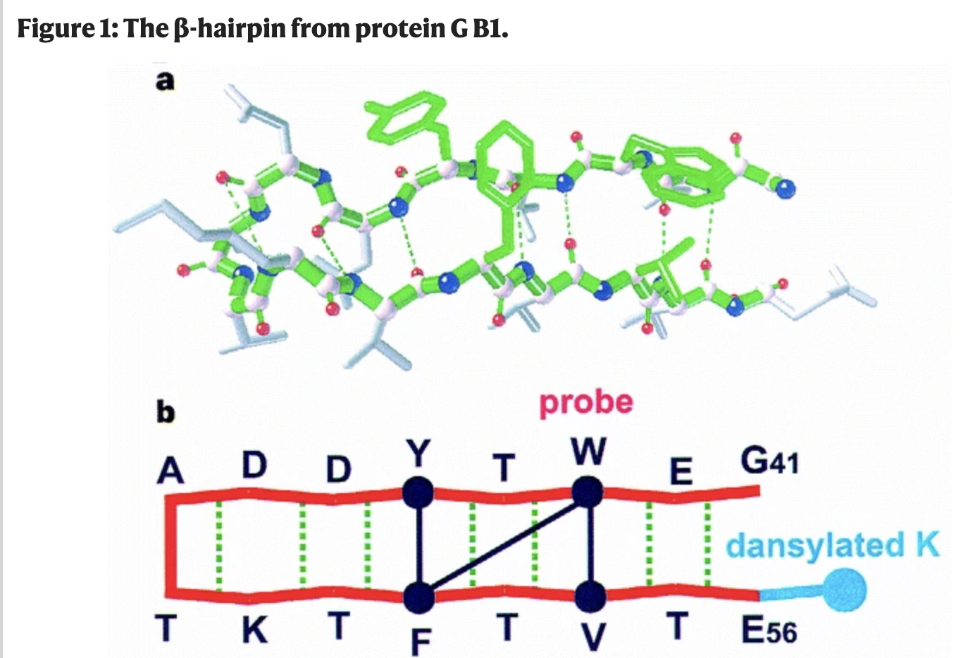
To understand our experiments, it helps to understand more about the protein folding task. The input is a sequence of amino acids (20 types like A, R, N, K) which we call "residues" when they are present in a protein. The output is a shape where each atom in a residue is given a precise location and orientation in 3D space, showing how the protein folds. Biologists often visualize a folded protein using a cartoon diagram like this:
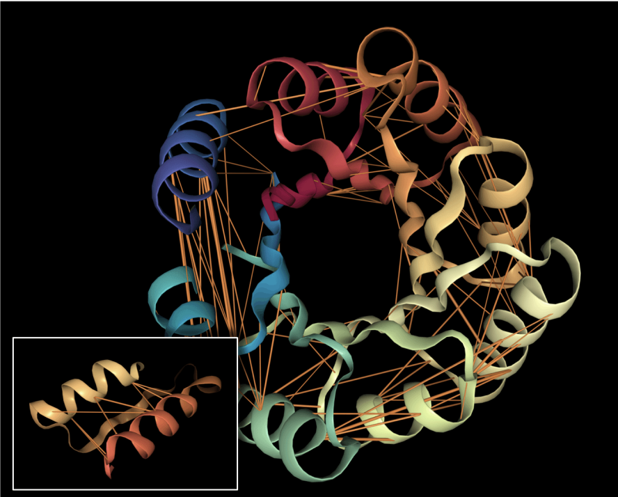
In our experiments, we study how the model folds a simple structural motif: the beta hairpin. A beta hairpin consists of two strands that run in opposite directions, connected by a tight turn and held together by affinities between matching residues on either side of the fold.
What is inside an AI Protein Folding Model?
ESMFold [Lin et al., 2023] predicts protein structure from sequence alone using a three-module architecture:
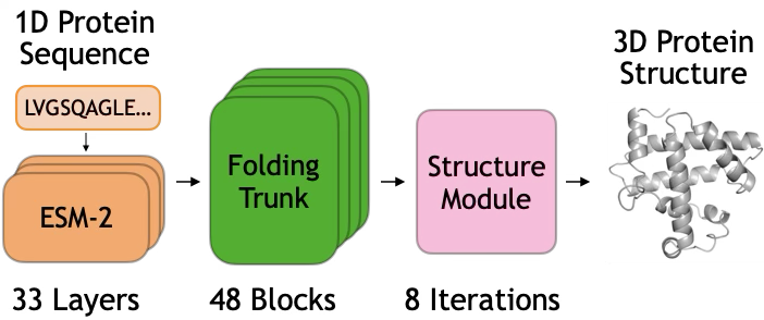
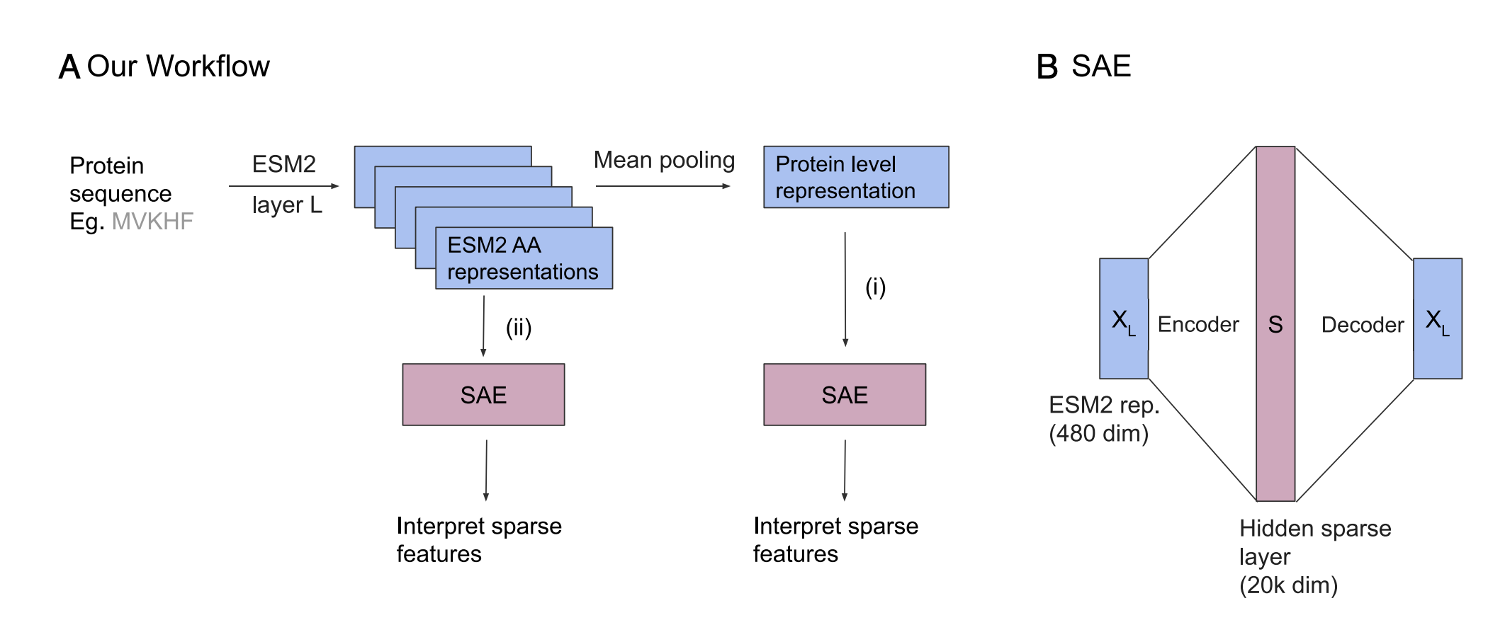
Module 1: ESM-2 Language Model. The input sequence is first processed by ESM-2, a 3B-parameter transformer pretrained on 250M protein sequences. ESM-2 produces a contextualized embedding $s_i \in \mathbb{R}^{2560}$ for each residue position $i$, capturing evolutionary and structural patterns learned during pretraining.
Module 2: Folding Trunk. The core of ESMFold is a folding trunk consisting of 48 stacked blocks. Each block maintains two representations:
- Sequence representation $s_i$ (per-residue features)
- Pairwise representation $z_{ij}$ (features for each residue pair)
Attention and Triangular Updates: Within each block, the sequence representation is updated via self-attention, while the pairwise representation is refined through triangular multiplicative updates (inspired by AlphaFold2) and row/column-based attention. The two representations are also coupled: each block exchanges information between them.
Module 3: Structure Module. After 48 folding blocks, the final pairwise representation $z_{ij}$ is passed to a structure module that predicts 3D coordinates.
When Does the Model Fold a Hairpin?
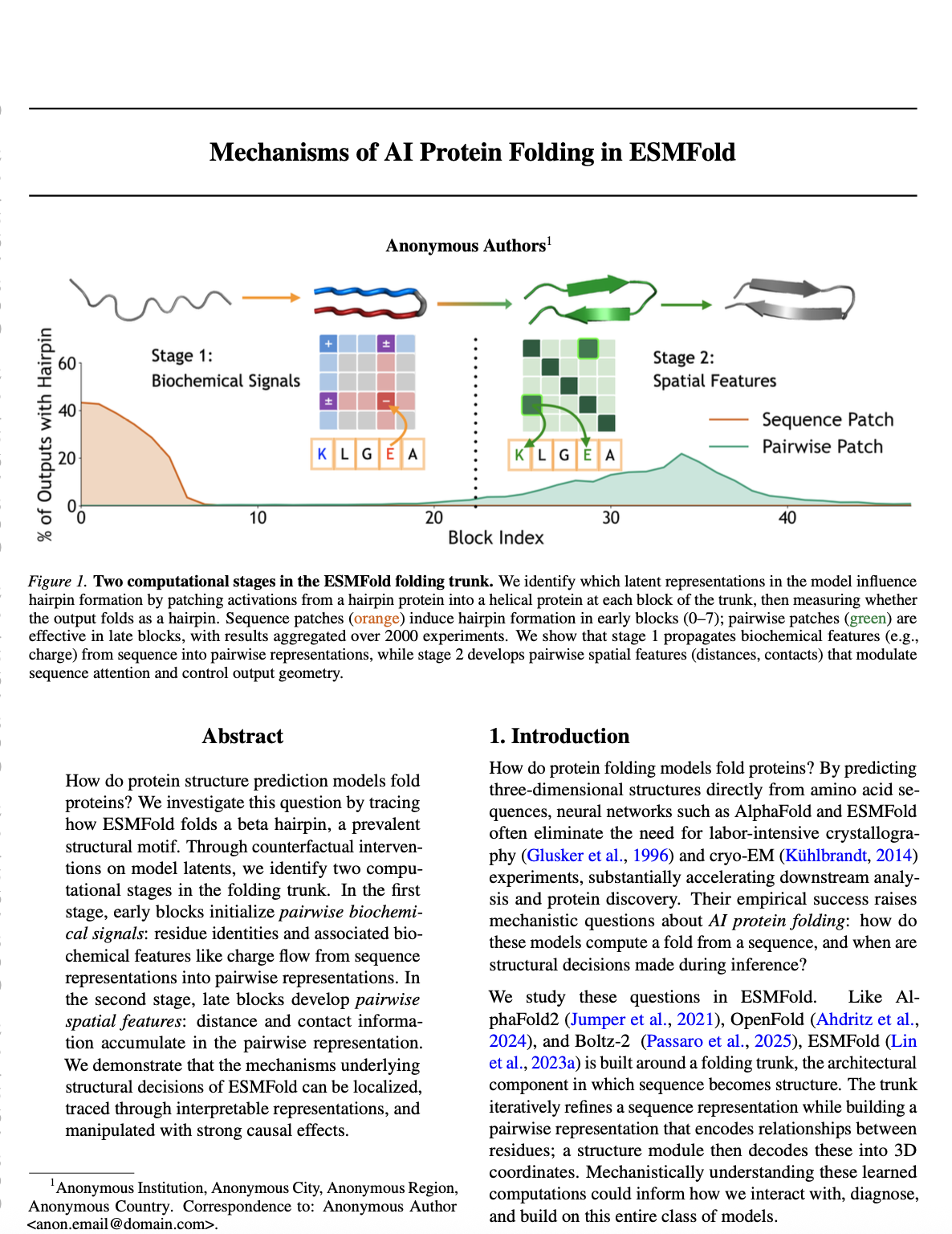
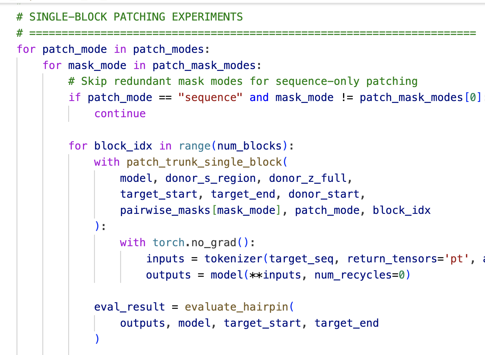
We use activation patching to localize where hairpin formation is computed in the folding trunk. We select a donor protein containing a beta hairpin and a target protein containing a helix-turn-helix motif. We run both proteins through ESMFold, extracting the sequence representation $s$ and pairwise representation $z$ at each block of the folding trunk. During the target's forward pass, we replace representations in the target's helical region with the donor's hairpin representations, aligning the two regions at their loop positions. We then observe whether the output structure contains a hairpin in the patched region.
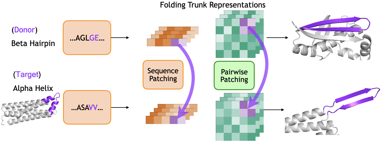
Single-block patching reveals two regimes (Figure 1). To localize the computation, we patch at a single block $k$, patching either sequence or pairwise representations alone. Restricting to the ~2,000 cases where full patching succeeded, we measure the success rate for each block and representation type:
- Sequence patches are effective in early blocks (0-7), with success rates peaking around 40% at block 0 and declining thereafter.
- Pairwise patches show the opposite pattern: they only become effective starting around block 25, reaching success rates around 20% by block 35.
We then investigate two distinct computational mechanisms: biochemical sequence information flow in early blocks, and spatial feature formation in late blocks.
ESMFold Learns and Uses Representations of Charge
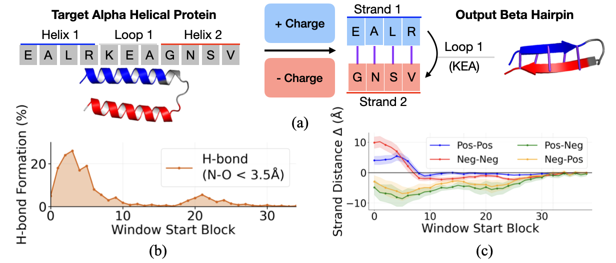
We ask whether the model leverages biochemical features to guide folding, and focus on charge. Charge is biochemically relevant for hairpin stability: antiparallel beta strands are often stabilized by salt bridges between oppositely charged residues on facing positions.
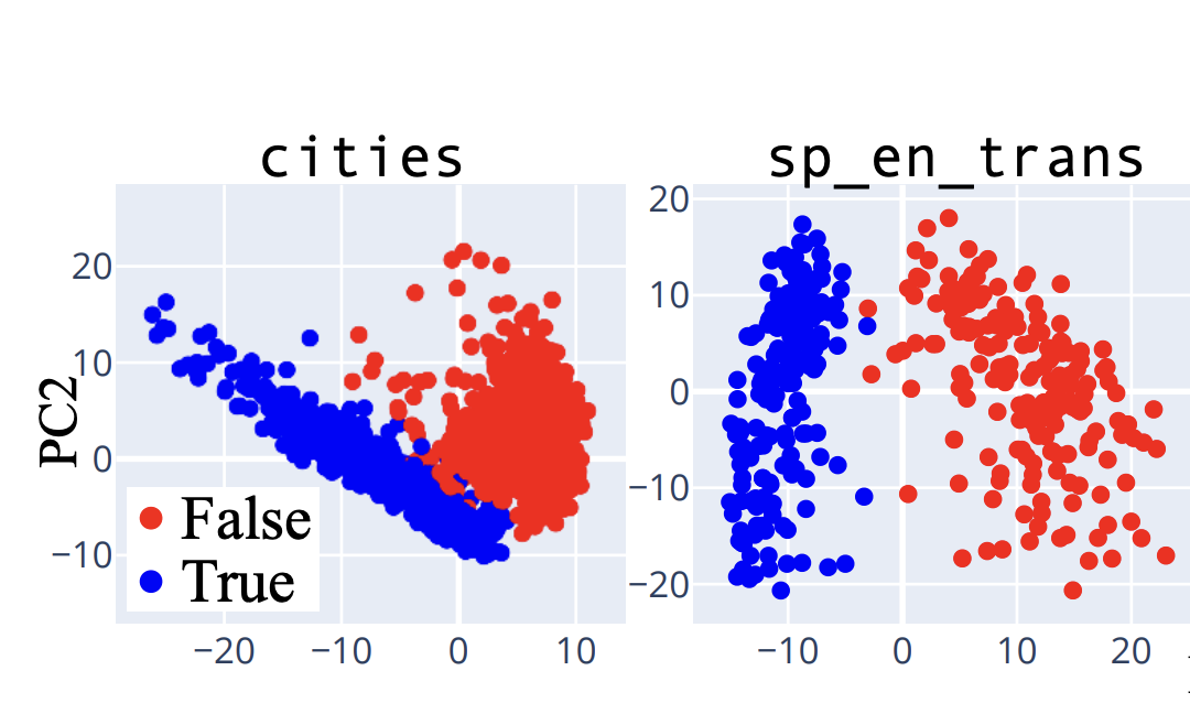
Charge is linearly encoded. We use a difference-in-means approach to identify a "charge direction" in the sequence representation space. Let $\mathcal{P} = \{\text{K}, \text{R}, \text{H}\}$ denote positively charged residues and $\mathcal{N} = \{\text{D}, \text{E}\}$ denote negatively charged residues. We compute:
$$v_{\text{charge}} = \frac{\bar{s}_{\mathcal{P}} - \bar{s}_{\mathcal{N}}}{\|\bar{s}_{\mathcal{P}} - \bar{s}_{\mathcal{N}}\|}$$Projecting residue representations onto $v_{\text{charge}}$ shows clean separation between charge classes at early blocks, confirming that charge is linearly encoded.
Electrostatic complementarity steering. Because this direction is linear, we can manipulate it. For a target helix-turn-helix region, we steer one helix toward positive charge and the other toward negative charge, mimicking the electrostatic complementarity of natural hairpins:
$$s_i' = s_i \pm \alpha \cdot v_{\text{charge}}$$Result: Complementarity steering induces hydrogen bond formation, with the effect concentrated in early blocks (0–10). As a control, steering both strands to the same charge increases cross-strand distance (repulsion), while opposite charges decrease it (attraction). This confirms that the charge direction causally influences predicted geometry.
We Can Manipulate Linear Representations of Residue Distances In ESMFold
By the late blocks, sequence patching no longer induces hairpin formation, but pairwise patching does. This suggests that the pairwise representation $z$ has taken over as the primary carrier of folding-relevant information. We hypothesize that $z$ encodes spatial relationships: particularly pairwise distances.
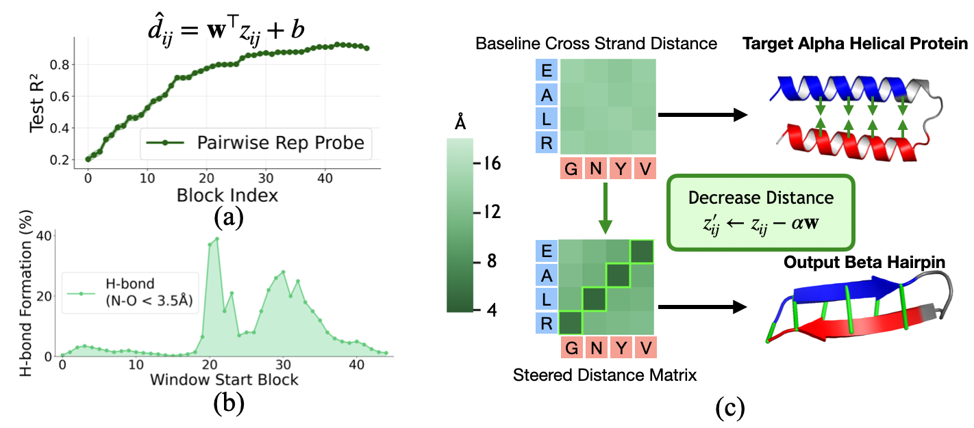
Distance probing. We train linear probes to predict pairwise C$_\alpha$ distance from $z$ at each block. Even at block 0, $z$ contains some distance information from positional embeddings. But as $z$ is populated with sequence information and refined through triangular updates, probe accuracy increases substantially, reaching $R^2 \approx 0.9$ by late blocks.
Distance steering. Since the probe is linear, we can steer toward a target distance (5.5Å, the typical C$_\alpha$–C$_\alpha$ spacing for cross-strand contacts in beta-sheets) by moving along the probe's weight direction:
$$z'_{ij} = z_{ij} - \alpha \cdot \mathbf{w}$$Result: Steering in blocks 20–35 is most effective, with hydrogen bond formation peaking around 40%. Steering in early blocks is less effective both because probes are less accurate and because subsequent computation can overwrite the perturbation. This confirms that late $z$ causally determines geometric outputs.
Pair2Seq Promotes Contact Information
How does distance information in $z$ influence the rest of the computation? The pair2seq pathway projects $z$ to produce a scalar bias that modulates sequence self-attention.
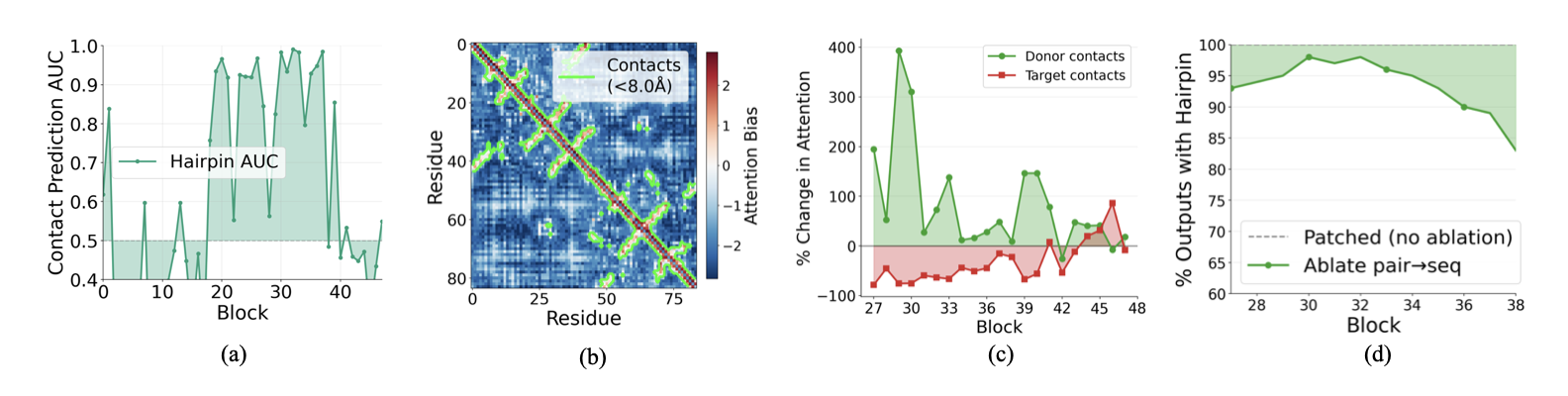
Bias encodes contacts. In middle and late blocks, the pair2seq bias cleanly separates contacting residue pairs (C$_\alpha$ distance < 8Å) from non-contacts (Fig. 6a). Residue pairs in contact receive substantially more positive bias than non-contacts, encouraging the sequence attention to preferentially mix information between contacting residues. We visualize the bias values across blocks in the Appendix, along with per-head biases which show distinct patterns and suggest head specialization as an area for future investigation.
Causal role. We tested this by patching the pairwise representation at block 27 and measuring how sequence attention changes. After patching, attention to donor-unique contacts increases substantially (up to 400%), while attention to target-unique contacts decreases. The pairwise representation causally redirects which residues attend to each other.
The Structure Module Uses Z as a Distance Map
The pair2seq pathway is one route by which $z$ influences the output. But $z$ also feeds directly into the structure module, which produces the final 3D coordinates.
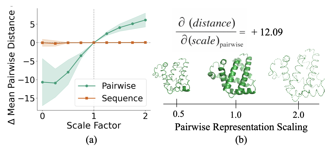
Scaling experiment. We scaled the pairwise representation by factors ranging from 0 to 2 before it enters the structure module, while holding $s$ fixed. We then repeated the experiment scaling $s$ while holding $z$ fixed.
Result: Scaling $z$ monotonically scales the mean pairwise distance between residues in the output structure. Scaling up causes the protein to expand; scaling down causes it to contract. In contrast, scaling $s$ has virtually no effect on output geometry. Together with our steering experiments, this confirms that $z$ acts as a geometric blueprint that the structure module renders into 3D coordinates.
Discussion
Protein folding models contain generalized knowledge that extends beyond their ability to output structures. Interpretability offers a way to unlock this knowledge: by extracting the biochemical principles these models have learned, by diagnosing the origins of prediction errors, and by redirecting model capabilities toward tasks they were not explicitly trained for: such as steering developability properties for protein design. Understanding how these models fold proteins, not just that they can, is a step toward making them even more effective scientific tools.
Related Work
Protein Structure Prediction
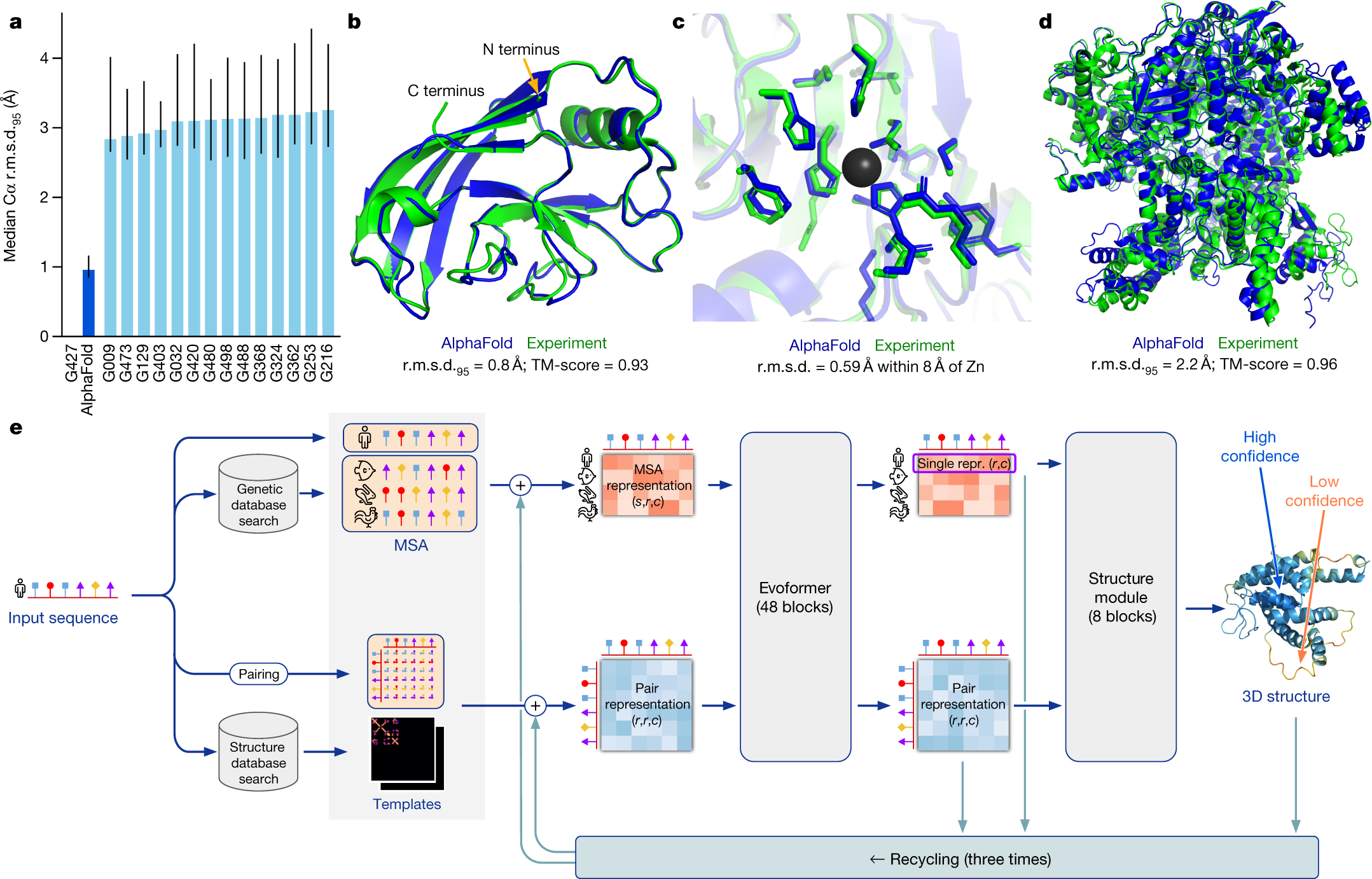
Highly Accurate Protein Structure Prediction with AlphaFold
Nature, 596, 583–589, 2021
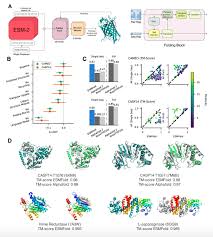
Evolutionary-Scale Prediction of Atomic-Level Protein Structure with a Language Model
Science, 379(6637), 1123–1130, 2023
Boltz-2: Towards Accurate and Efficient Binding Affinity Prediction
bioRxiv preprint, 2025
Mechanistic Interpretability
First Conference on Language Modeling, 2024
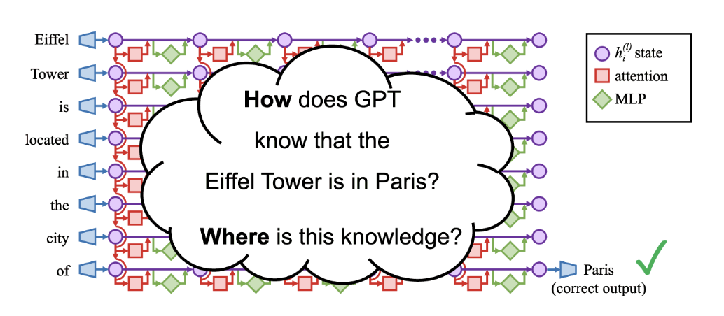
Locating and Editing Factual Associations in GPT
Advances in Neural Information Processing Systems (NeurIPS), 2022
Mechanistic Interpretability in Biology
Proceedings of the National Academy of Sciences (PNAS), 2025
Protein Folding Biology
Folding Dynamics and Mechanism of β-Hairpin Formation
Nature, 390, 196–199, 1997
Annual Review of Biophysics, 37, 289–316, 2008
How to cite
The paper can be cited as follows.
bibliography
Lu, K., Brinkmann, J., Huber, S., Mueller, A., Belinkov, Y., Bau, D., & Wendler, C. (2026). Mechanisms of AI Protein Folding in ESMFold. arXiv preprint arXiv:2602.06020.
bibtex
@article{lu2026mechanisms,
  title={Mechanisms of AI Protein Folding in ESMFold},
  author={Lu, Kevin and Brinkmann, Jannik and Huber, Stefan and Mueller, Aaron and Belinkov, Yonatan and Bau, David and Wendler, Chris},
  journal={arXiv preprint arXiv:2602.06020},
  year={2026}
}
Appendix: Bias Maps
We visualize the pair2seq attention bias across blocks and across individual attention heads. For a single protein (PDB: 6rwc), we extract the bias term $\beta_{ij}(z_{ij})$ and average over heads. Green contours indicate structural contacts (C$_\alpha$ distance < 8Å).
Bias Across Blocks (Head-Averaged)
Each panel shows the bias term $\beta_{ij}$, averaged across all 8 attention heads, for protein 6rwc at selected blocks of the folding trunk. Red indicates positive bias (encouraging attention); blue indicates negative bias. In early blocks, the bias is near-uniform; by the middle blocks, it begins to align with the contact map, and by late blocks, contacting residue pairs receive substantially higher bias than non-contacts.
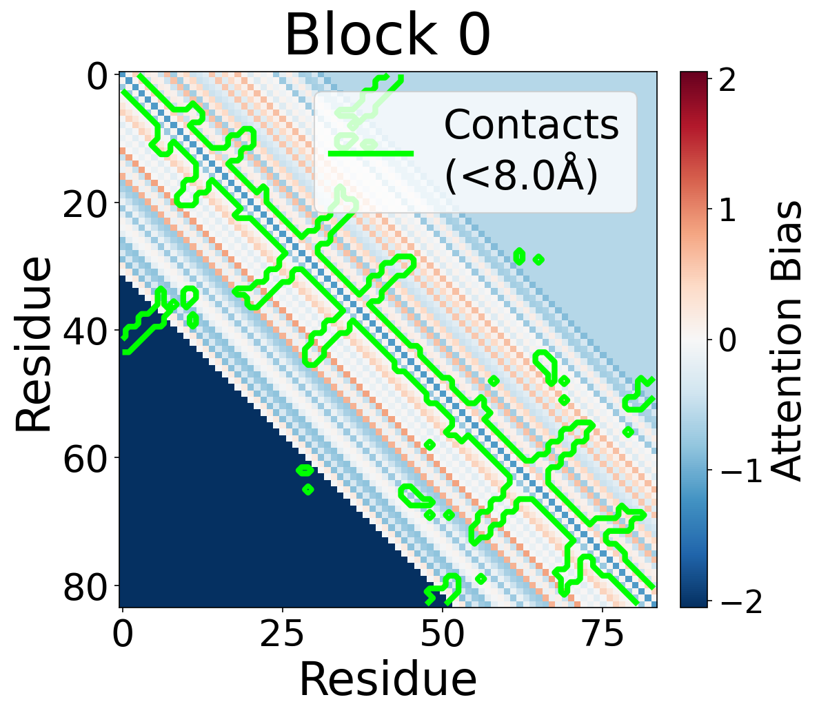
Block 0
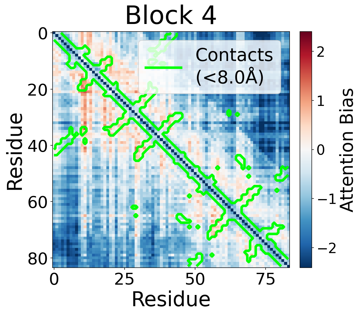
Block 4
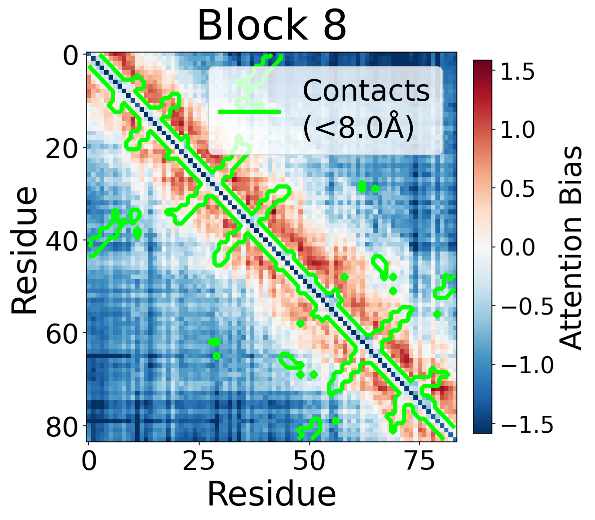
Block 8
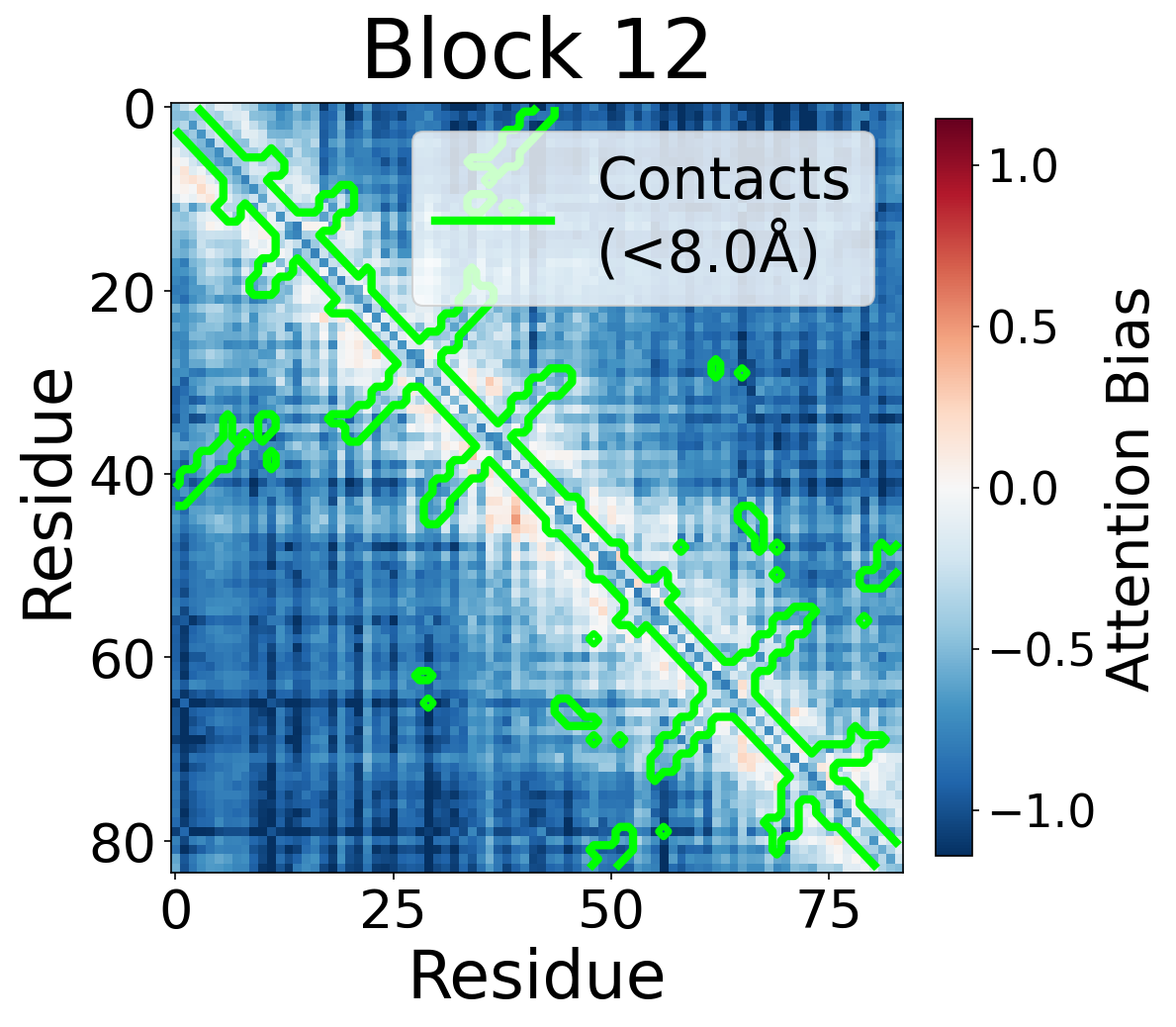
Block 12
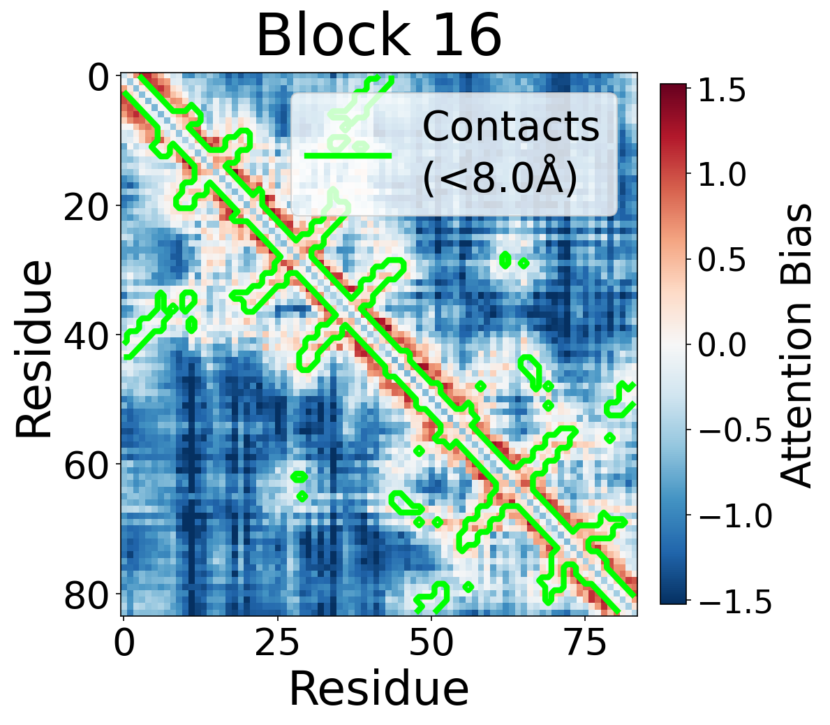
Block 16
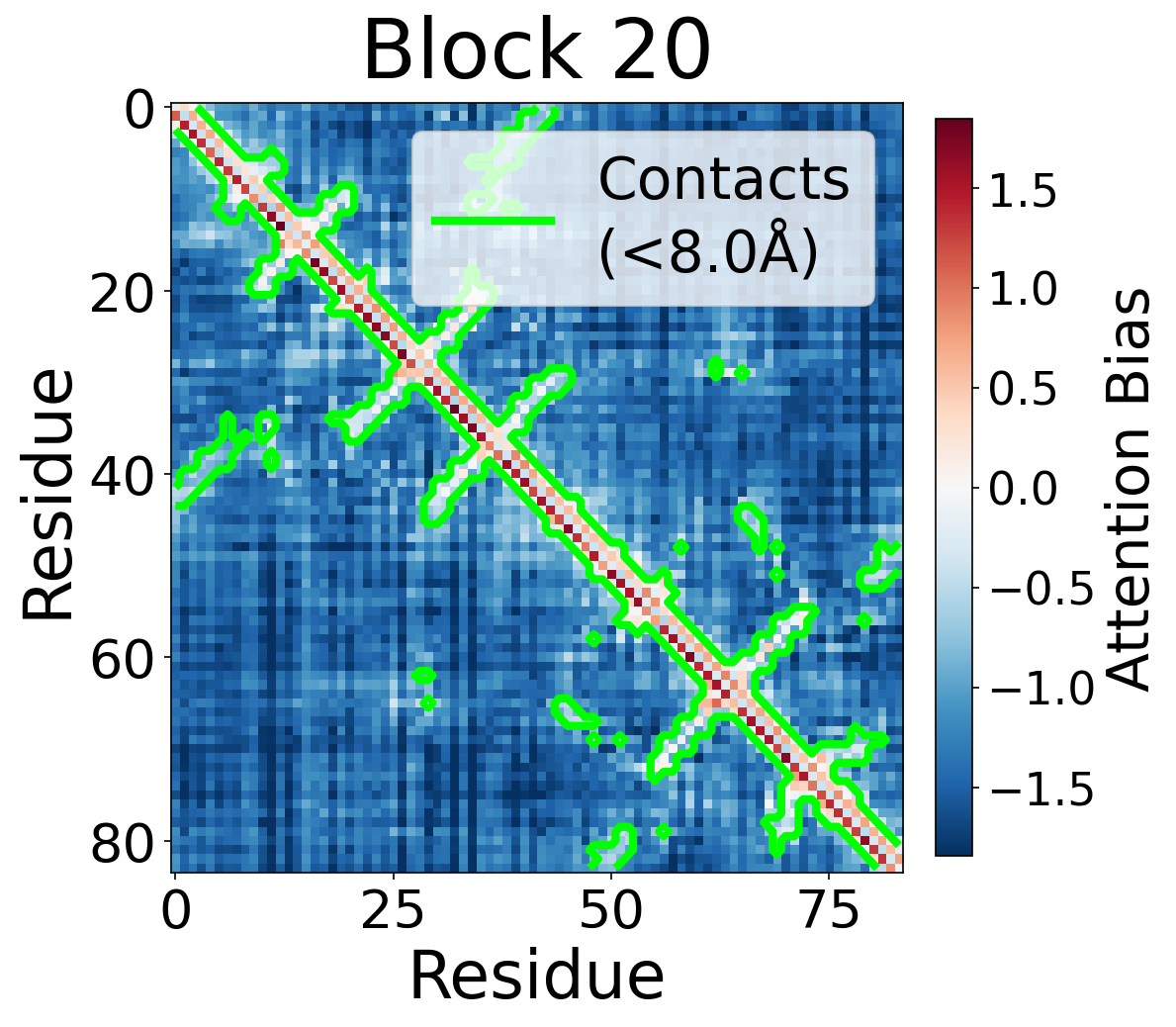
Block 20
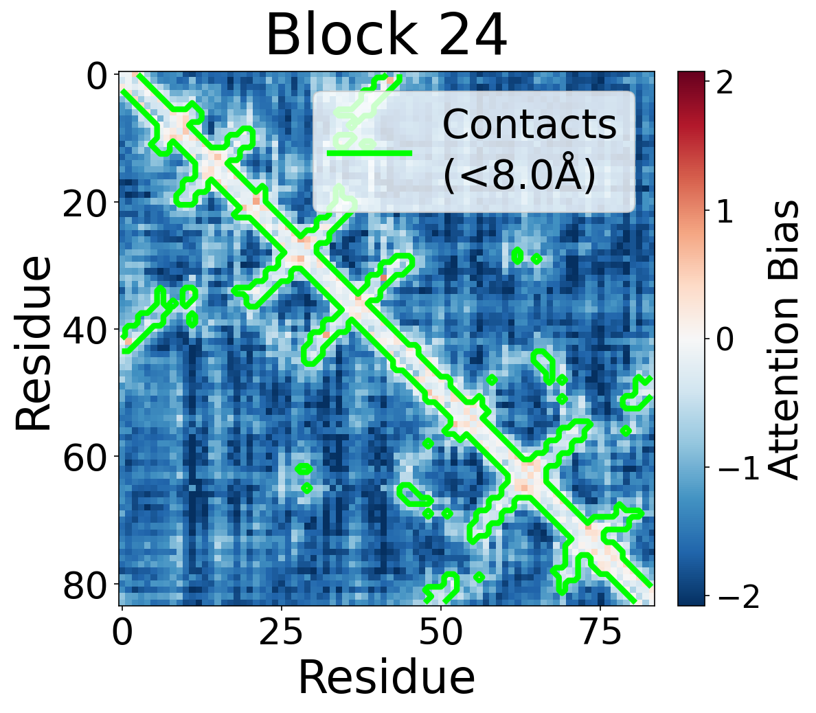
Block 24
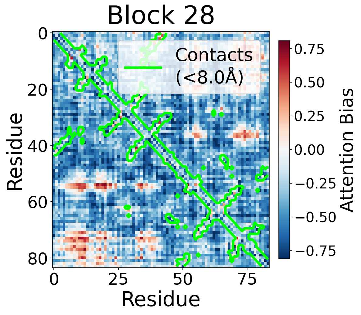
Block 28
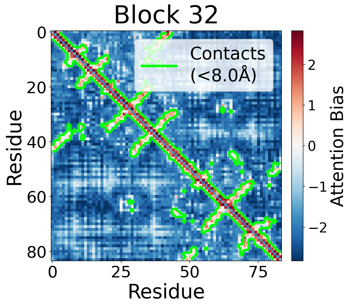
Block 32
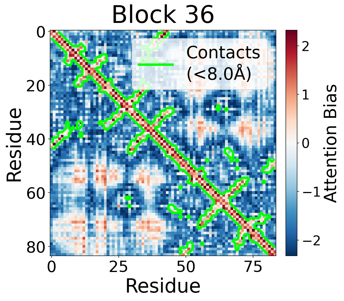
Block 36
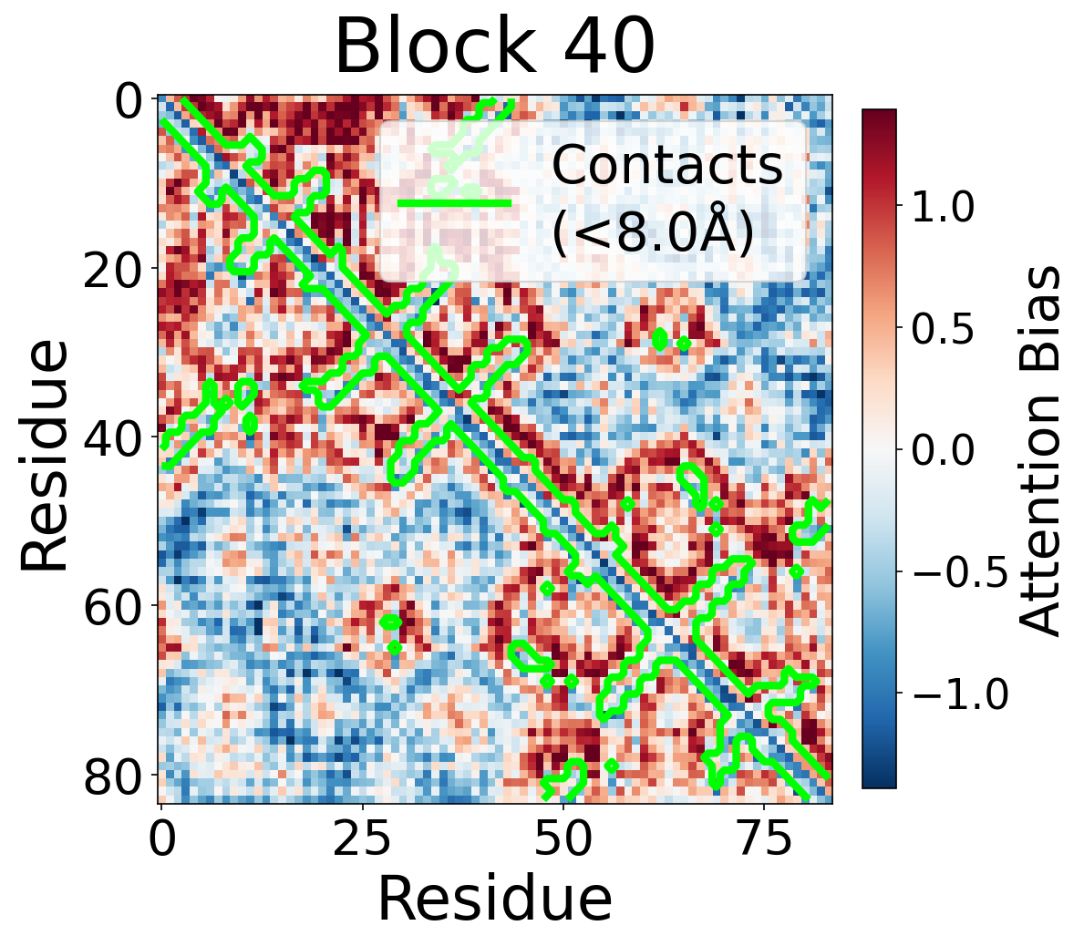
Block 40
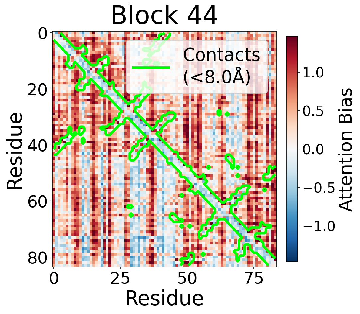
Block 44
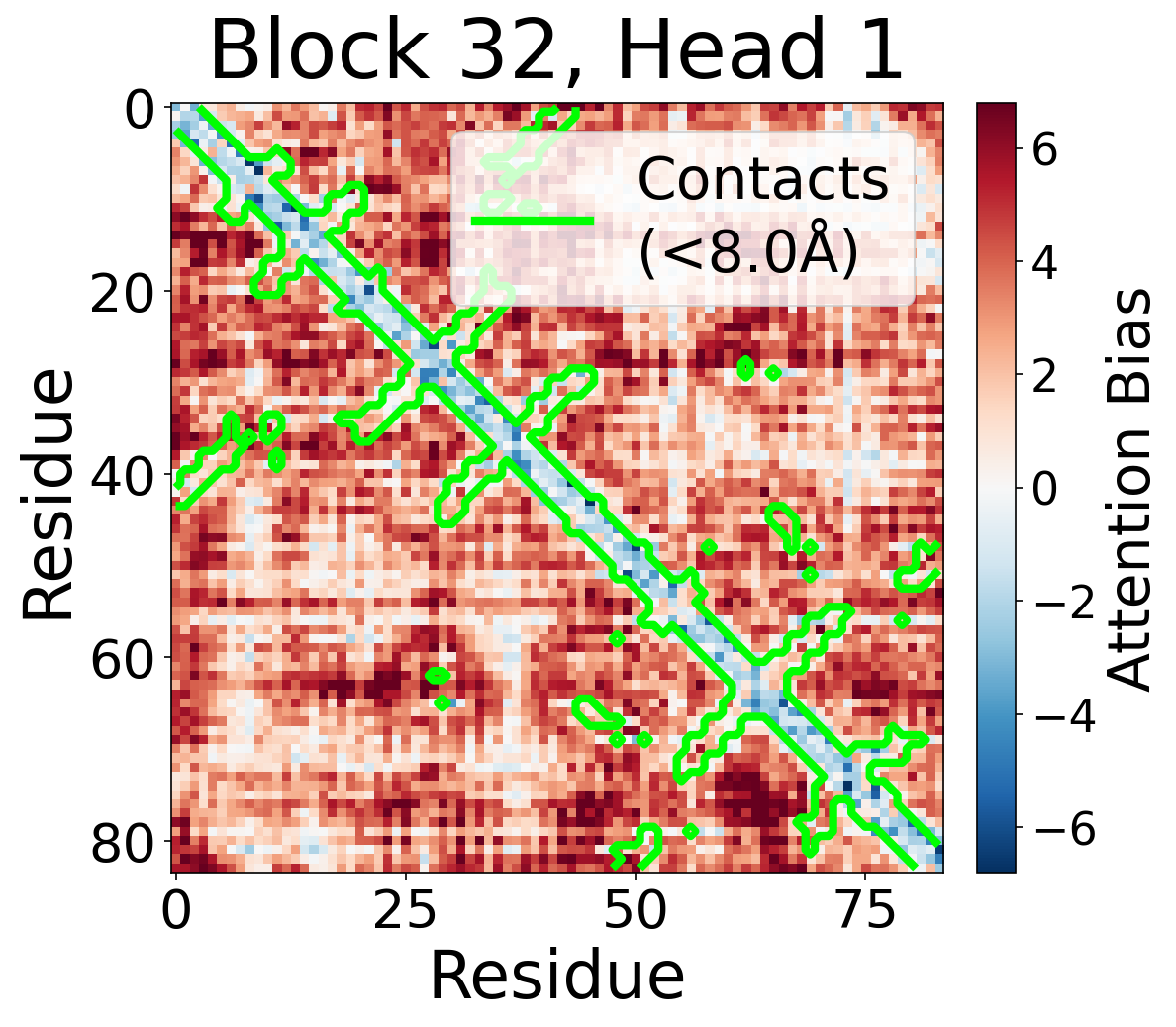
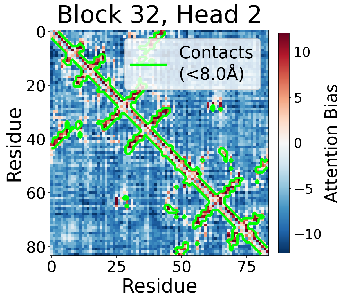
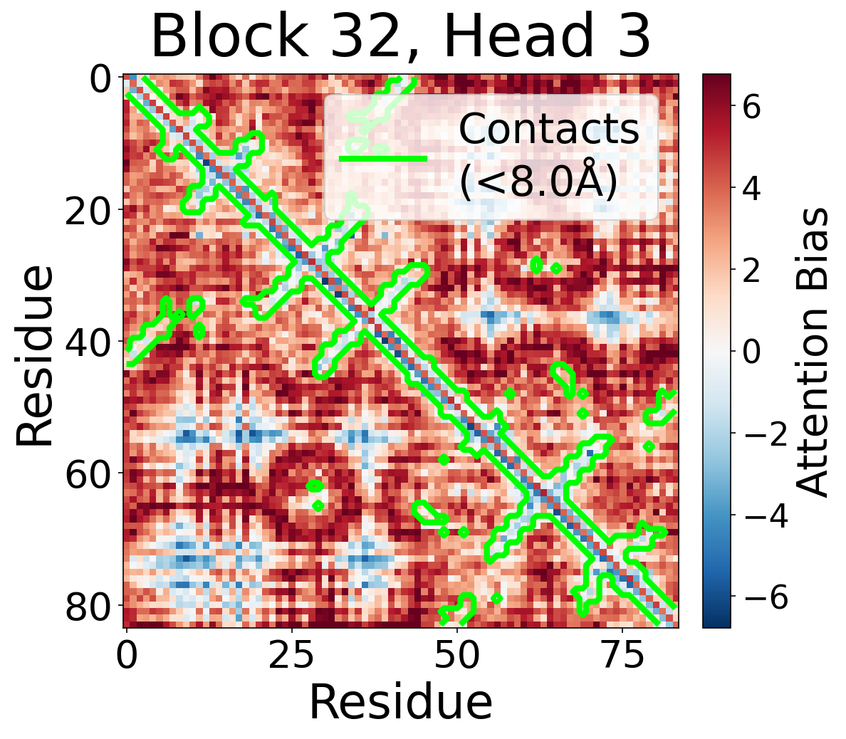
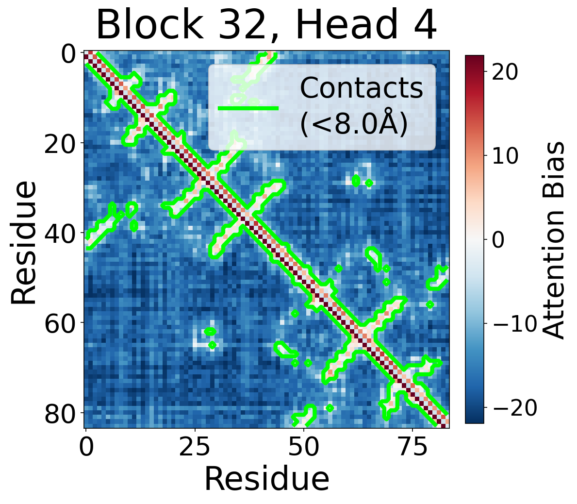
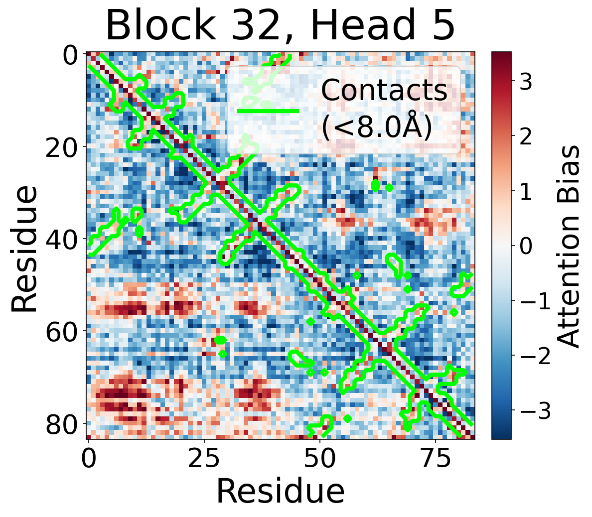
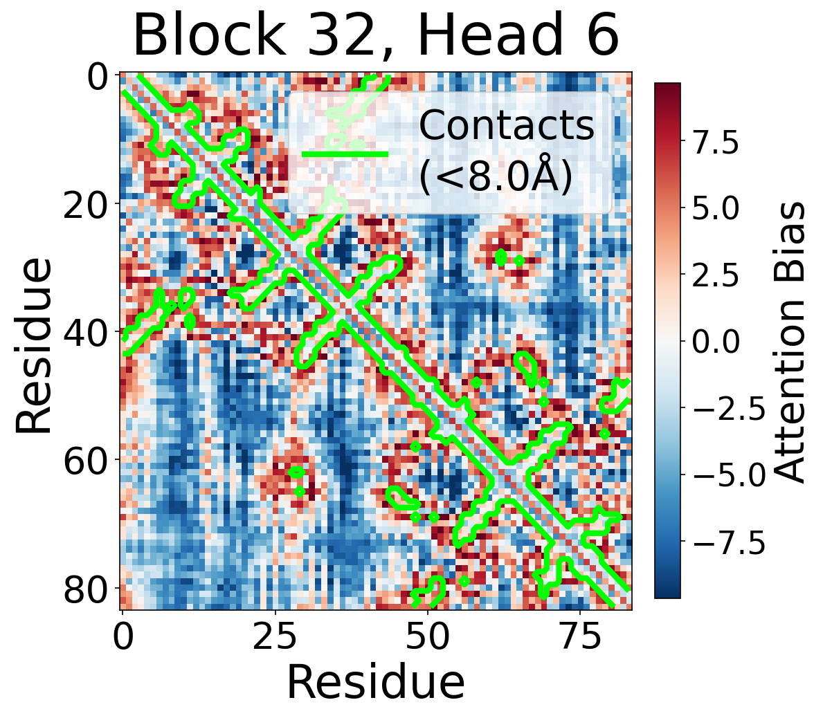
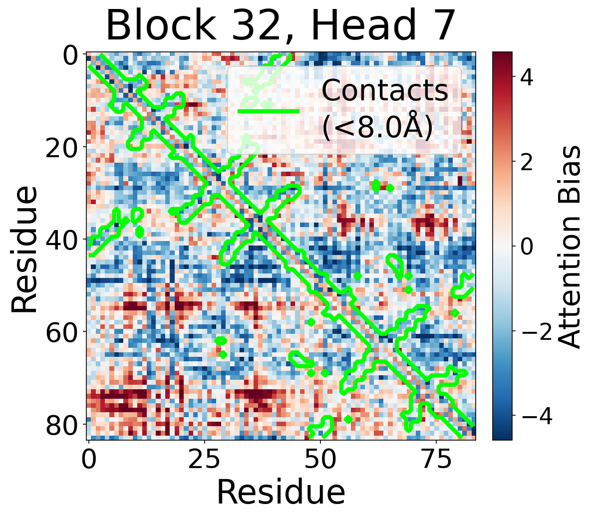
Per-Head Bias at Block 32
Individual attention head bias values for protein 6rwc at block 32. Different heads exhibit distinct patterns: some heads show strong contact-aligned bias, while others capture different spatial relationships or show more diffuse patterns. Block 32 head 2 and head 4 generally show this specialized pattern across different protein types, suggesting that individual heads attend to complementary aspects of pairwise geometry.
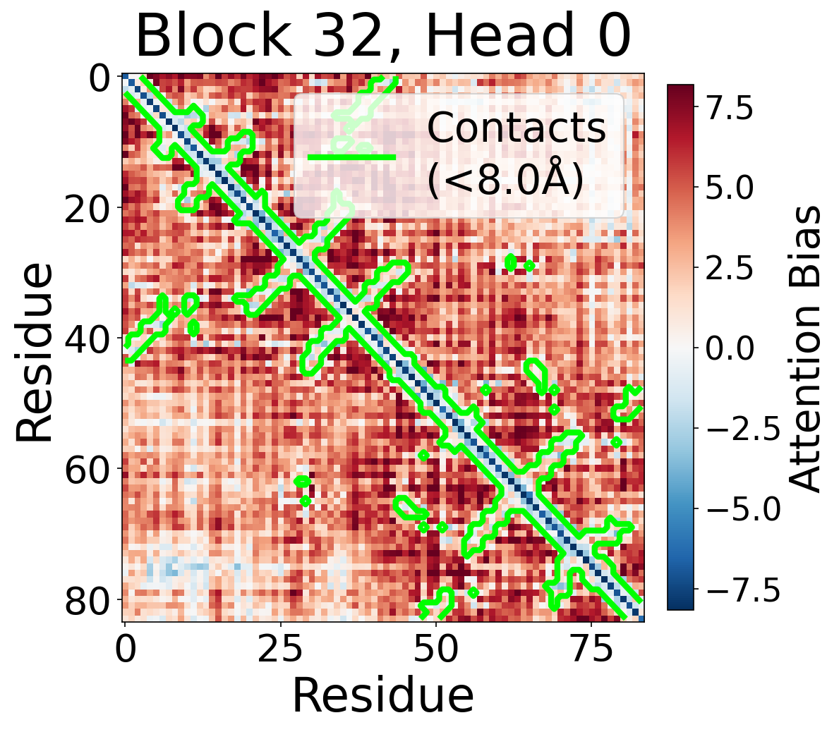
Head 0
Head 1
Head 2
Head 3
Head 4
Head 5
Head 6
Head 7